Graph Pooling
Published:
Given the node embeddings of a graph, how can we make predictions at graph-level?
$\rightarrow$ We will have to learn the embedding for the entire a graph by pooling node embeddings and this is usually referred as graph pooling.
In this blog, I will break down some strategies for graph pooling.
I will present a graph as $\mathcal{G} = (V, E)$, where $V$ the set of nodes and $E$ is the set of edges. I denote the adjacency matrix and node embeddings as $\mathbf{A} \in \mathbb{R}^{ \vert V \vert \times \vert V \vert}$, $\mathbf{Z} \in \mathbb{R}^{\vert V \vert \times d}$ respectively.
Table of Contents
Set Pooling Methods
The goal Set Pooling is to map a set of node embeddings \(\{\mathbf{z}_{1}, \ldots, \mathbf{z}_{\vert V \vert}\}\) to an embedding that represents the entire graph, \(\mathbf{z}_{G}\).
Global pooling
We can obtain the embedding for the graph by taking the sum, mean, or max of node embeddings.
We can use this method for small graphs.
Set2Set
Vinyals et al. Order matters: Sequence to sequence for sets, ICLR 2015
This method allows us to pool node embeddings using LSTMs and attention.
Set2Set iterates for $t = 1, \dots, T$ steps
At step $t$:
- Compute the query vector for attention at iteration $t$
- Compute the attention score over each node using the attention function $f_a: \mathbb{R}^d \times \mathbb{R}^d \rightarrow \mathbb{R}$
- Normalize the attention score to obtain the attention weights
- Compute the weighted sum of node embeddings, the weight for each node’s embedding is its attention weight computed in the previous step
After $T$ iterations, compute the final embedding of the graph by the following equation:
\[\mathbf{z}_G = \text{CONCAT}(\mathbf{o}_1, \dots, \mathbf{o}_T)\]Graph Coarsening Methods
A drawback of Set Pooling Methods is that they do not exploit the structure of the graph (They compute the graph embedding solely based on node embeddings).
A strategy for taking graph structure into account is performing graph coarsening / clustering while pooling node representations.
Lets say we want to group nodes into $c$ clusters. We will use a clustering function
\[f_c: \mathcal{G} \times \mathbb{R}^{\vert V \vert \times d} \rightarrow \mathbb{R}^{\vert V \vert \times c}\]that maps nodes to an assignment matrix over $c$ clusters.
Suppose we have a cluster assignment matrix
\[\mathbf{S} = f_c(\mathcal{G}, \mathbf{Z}) \in \mathbb{R}^{\vert V \vert \times c}\]where $\mathbf{S}_{v, i}$ denotes how likely node $v$ is in cluster $i$
We will use $\mathbf{S}$ to coarsen the graph. Specifically, we will compute the coarsened adjacency matrix
\[\mathbf{\hat{A}} = \mathbf{S}^T \mathbf{A} \mathbf{S} \in \mathbb{R}^{c\times c}\]and a new matrix of embeddings
\[\mathbf{\hat{X}} = \mathbf{S}^T \mathbf{Z} \in \mathbb{R}^{c \times d}\]Intuition of $\mathbf{\hat{A}}$ and $\mathbf{\hat{X}}$
\[\mathbf{\hat{A}}_{i, j} = \sum_{v \in V} \sum_{u \in N(v)} \mathbf{S}_{v, i} \mathbf{S}_{u,j}\]
For $i, j \leq c$Therefore, $\mathbf{\hat{A}}_{i, j} \in \mathbb{R}$ represents the weight of connections (edges) between cluster $i$ and cluster $j$. In other words, $\mathbf{\hat{A}}$ represents the strength of connections between each pair of $c$ clusters. ($\mathbf{\hat{A}}$ is the weighted adjacency matrix of the coarsened graph)
$\mathbf{\hat{X}}$ takes in the node embeddings, $\mathbf{Z}$, aggregrates them base on the assignment matrix $\mathbf{S}$, and outputs pooled features for clusters (the $i$-th row of $\mathbf{\hat{X}}$ represents the features of cluster $i$).
After grouping the nodes into $c$ clusters, we will obtain a coarsened graph that has $c$ nodes (we just reduced the number of nodes to $c$ !!), which is represented by the weighted adjacency matrix $\mathbf{\hat{A}}$, and new node features $\mathbf{X}$. Then we can apply GNN on this coarsened graph and repeat the whole process for $T$ times. Thus, after each iteration, the graph’s size will be reduced, and we will obtain the original graph’s embedding using node embeddings of the final coarsened graph.
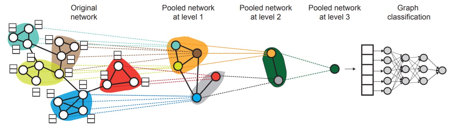
DiffPool
Ying et al. Hierarchical Graph Representation Learning with Differentiable Pooling, NeurIPS 2018
 From Source
DiffPool stacks $L$ GNN modules and learns to assign nodes to clusters at each layer using the embeddings of the previous layer. Therefore, DiffPool learns node embeddings that benefit both graph classification and hierarchical pooling.
DiffPool consists of 2 phases: Pooling nodes and Learning cluster assignment matrix
Pooling nodes
Denote the learned cluster assignment matrix at layer $l$ as $\mathbf{S}^{(l)} \in \mathbb{R}^{n_l \times n_{l + 1}}$, where $n_l$ is the number of nodes at layer $l$ and $n_{l + 1}$ is the number of nodes at layer $l + 1$. Denote the adjacency matrix and node embedding matrix at layer $l$ as $\mathbf{A}^{(l)} \in \mathbb{R}^{n_l \times n_l}$ and $\mathbf{Z}^{(l)} \in \mathbb{R}^{n_l \times d}$ respectively. DiffPool coarsens the graph at layer $l$ by the following equations:
\[\mathbf{A}^{(l + 1)} = \mathbf{S}^{(l)^T} \mathbf{A}^{(l)} \mathbf{S}^{(l)} \in \mathbb{R}^{n_{l + 1} \times n_{l + 1}}\] \[\mathbf{X}^{(l + 1)} = \mathbf{S}^{(l)} \mathbf{Z}^{(l)} \in \mathbb{R}^{n_{l + 1} \times d}\]$\mathbf{X}^{(l + 1)}$ and $\mathbf{A}^{(l + 1)}$ represent the node features and weighted adjacency matrix of the coarsened graph, which is the graph at layer $l + 1$. These two matrices will be used at inputs to layer $l + 1$.
Learning cluster assignment matrix
At layer $l$, given the coarsened adjacency matrix $\mathbf{A}^{(l)}$ and node features $\mathbf{X}^{(l)}$, how can we learn the assignment matrix $\mathbf{S}^{(l)}$ and the node embeddings $\mathbf{Z}^{(l)}$?
DiffPool uses 2 seperate GNNs to learn \(\mathbf{S}^{(l)}\) and \(\mathbf{Z}^{(l)}\), which is \(\text{GNN}^{(l)}_{pool}\) and \(\text{GNN}^{(l)}_{embed}\) respectively:
\[\mathbf{Z}^{(l)} = \text{GNN}^{(l)}_{embed} (\mathbf{A}^{(l)}, \mathbf{X}^{(l)})\]$\text{GNN}^{(l)}_{embed}$ uses the adjacency matrix $\mathbf{A}^{(l)}$ and node features $\mathbf{X}^{(l)}$ to generate node embeddings $\mathbf{Z}^{(l)}$
\[\mathbf{S}^{(l)} = \text{softmax}(\text{GNN}^{(l)}_{embed}(\mathbf{A}^{(l)}, \mathbf{S}^{(l)}))\]where $\text{softmax}$ is applied in the row-wise way, since $\mathbf{S}^{(l)}$ represents the probabilistic assignment for each node.
At layer $0$, the input will be the original graph’s adjacency matrix $\mathbf{A}$ and node features $\mathbf{X}$. At the second to last layer $L - 1$, we set the cluster assignment matrix $\mathbf{S}^{(L - 1)}$ to a vector of $1$’s, meaning that the nodes at layer $L - 1$ will be assigned into a single cluster, and layer $L$ will generate a final embedding vector, which represents the original graph’s embedding.
Permutation Invariance
In order to be used in graph classification, DiffPool should be permutation invariant.Proposition. Let $P$ be any permutation matrix. Then $\text{DiffPool}(\mathbf{A}, \mathbf{Z}) = \text{DiffPool}(P\mathbf{A} P^T, P \mathbf{Z})$ as long as $\text{GNN}(\mathbf{A}, \mathbf{X}) = \text{GNN}(P\mathbf{A} P^T, P \mathbf{X})$. ($\text{GNN}$ refers to the GNN module used in DiffPool)
Proof.
\[\begin{split} (\mathbf{S}, \mathbf{Z}) & = \text{GNN}(\mathbf{A}, \mathbf{X}) \\ (\mathbf{S}_P, \mathbf{Z}_P) & = \text{GNN}(P \mathbf{A} P^T, P \mathbf{X}) \\ (\mathbf{\hat{A}}, \mathbf{\hat{X}}) & = \text{DiffPool}(\mathbf{A}, \mathbf{Z}) \\ (\mathbf{\hat{A}}_P, \mathbf{\hat{X}}_P) & = \text{DiffPool}(P \mathbf{A} P^T, P \mathbf{Z}) \\ \end{split}\]
LetIn order to prove the the permutation invariance of $\text{DiffPool}$, we will prove that $\mathbf{S} = \mathbf{S}_P$, $\mathbf{Z} = \mathbf{Z}_P$, $\mathbf{\hat{A}} = \mathbf{\hat{A}}_P$, and $\mathbf{\hat{X}} = \mathbf{\hat{X}}_P$
Since $\text{GNN}(\mathbf{A}, \mathbf{X}) = \text{GNN}(P\mathbf{A} P^T, P \mathbf{X})$, $\mathbf{S} = \mathbf{S}_P$ and $\mathbf{Z} = \mathbf{Z}_P$.
We have
\[\begin{split} \mathbf{\hat{A}}_P & = (P \mathbf{S})^T(P\mathbf{A} P^T)(P\mathbf{S}) \\ & = \mathbf{S}^T(P^TP)\mathbf{A}(P^TP)\mathbf{S} \\ & = \mathbf{S}^T \mathbf{A} \mathbf{S} \text{ (since } P^TP = I)\\ & = \mathbf{\hat{A}} \\ \\ \mathbf{\hat{X}}_P & = (P\mathbf{S})^T(P \mathbf{Z}) \\ & = \mathbf{S}^T(P^TP)\mathbf{Z} \\ & = \mathbf{S}^T \mathbf{Z} \text{ (since } P^TP = I)\\ & = \mathbf{\hat{X}} \end{split}\]Thus, the proposition is proved.
Auxiliary Link Prediction Objective and Entropy Regularization
In pratice training the pooling GNN \((\text{GNN}_{pool})\) based only on gradient in the graph classification task can be difficult, since optimizing the \(\text{GNN}_{pool}\) will now become a non-convex optimization problem. In order to address this problem, the authors of DiffPool train \(\text{GNN}_{pool}\) with an auxiliary link prediction objective, which tells us that nearby nodes should be pooled together. Specifically, at each layer $l$, the following loss function will be minimized:
\[L_{LP} = \Vert \mathbf{A}^{(l)} - \mathbf{S}^{(l)} \mathbf{S}^{(l)^T} \Vert _F\]where $\Vert . \Vert _F$ denotes the Forbenius norm.
Intuition of $L_{LP}$
At each layer $l$, let $\mathbf{Q} = \mathbf{A}^{(l)} - \mathbf{S}^{(l)} \mathbf{S}^{(l)^T}$, then $L_{LP} = \sqrt{\sum_{i \in V} \sum_{j \in V} \mathbf{Q}_{ij}^2}$
We have \(\mathbf{Q}_{ij} = \mathbf{A}^{(l)}_{ij} - \mathbf{S}^{(l)}_i \mathbf{S}^{(l)^T}_j\), where \(\mathbf{S}^{(l)}_i\) is the \(i\)-th row of \(\mathbf{S}^{(l)}\).
Thus, minimizing $L_{LP}$ means minimizing $\sum_{i \in V} \sum_{j \in V} (\mathbf{A}^{(l)}_{ij} - \mathbf{S}^{(l)}_i \mathbf{S}^{(l)^T}_j)^2 $.
If $i$ and $j$ are nearby then both \(\mathbf{A}^{(l)}_{ij}\) and \(\mathbf{S}^{(l)}_i \mathbf{S}^{(l)^T}_j\) will be large. Similarly, if \(i\) and \(j\) are not nearby then both \(\mathbf{A}^{(l)}_{ij}\) and \(\mathbf{S}^{(l)}_i \mathbf{S}^{(l)^T}_j\) will be small. Thus minimizing \(L_{LP}\) will force nearby nodes being pooled together.
Moreover, the cluster assignment matrix $\mathbf{S}^{(l)}$ learned by the pooling GNN should have row vectors that are close to one-hot vectors, so that the node assignment can be clearly defined. Therefore, the authors of DiffPool regularize the entropy of the cluster assignment by minimizing the following equation:
\[L_E = \frac{1}{\vert V \vert} \sum_{i \in V}H(\mathbf{S}^{(l)}_i)\]where $H$ is the entropy function.
Intuition of $L_E$
Minimizing $L_E$ will minimize the entropy of the cluster assignment of each node, i.e forcing $\text{GNN}_{pool}$ to be confidence about assigning each node into a cluster.
During training, $L_{LP}$ and $L_E$ of each layer will be added to the classification loss.
Top-$K$ methods
Unlike Graph Coarsening Methods, instead of clustering nodes, Top-$K$ methods rank nodes and select nodes with top $k$ score. The selected nodes then will form a new graph.
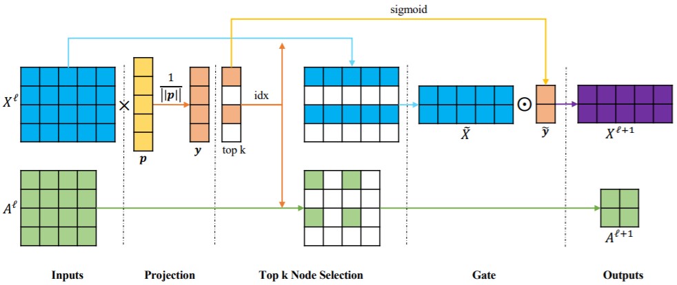
gPool
H. Gao, S. Ji. Graph U-Nets, ICML 2019
 From Source
gPool layer selects a new subset of nodes of the original graph to form a new and smaller graph. gPool consists of 3 phases: Projection, Node Selection, and Gate
Denote the number of nodes in the graph at layer $l$ as $n_l$. Denote the graph’s adjacency matrix and node features at gPool layer $l$ as $\mathbf{A}^{(l)} \in \mathbb{R}^{n_l \times n_l}$ and $\mathbf{X}^{(l)} \in \mathbb{R}^{n_l \times d}$ respectively.
Projection
gPool layer $l$ learns a projection vector $\mathbf{p}^{(l)} \in \mathbb{R}^{n_l \times 1}$ to and projects node features $\mathbf{X}^{(l)}$ to 1 dimension:
\[\mathbf{y} = \mathbf{X}^{(l)} \frac{\mathbf{p}^{(l)}}{\Vert \mathbf{p}^{(l)} \Vert} \in \mathbb{R}^{n_l \times 1},\]where $\mathbf{y}_i \in \mathbb{R}$ is node $i$’s score and it represents how much information of node $i$ can be retained when we project node $i$’s features onto the dimension of $\mathbf{p}^{(l)}$
Node Selection
Since we want to preserve as much information as possible, we select $k$ nodes with the highest score and record their indices:
\[\text{idx} = \text{rank}(\mathbf{y}, k)\]After selecting $k$ nodes, we obtain a new graph represented by a new adjacency matrix $\mathbf{\hat{A}}$ and new node features $\mathbf{\hat{X}}$. Specifically, based on the indices of selected nodes, gPool extracts some rows and columns of $\mathbf{A}$ to form $\mathbf{\hat{A}}$ and extracts some rows of $\mathbf{X}$ to form $\mathbf{\hat{X}}$:
\[\mathbf{A}^{(l + 1)} = \mathbf{\hat{A}} = \mathbf{A}^{(l)}(\text{idx}, \text{idx}) \in \mathbb{R}^{k \times k}\] \[\mathbf{\hat{X}} = \mathbf{X}^{(l)}(\text{idx}, :) \in \mathbb{R}^{k \times d}\]Gate
In order to control the information flow, gPool applies gate operation:
\[\mathbf{\hat{y}} = \sigma(\mathbf{y}(\text{idx})),\]where $\sigma(.)$ is the sigmoid function
\[\mathbf{X}^{(l + 1)} = \mathbf{\hat{X}} \odot (\mathbf{\hat{y}} \mathbf{1}_d^T),\]where $\odot$ is the element-wise matrix product
Applying the gate operator, gPool makes the projection vector $\mathbf{p}^{(l)}$ trainable by back-propagation.
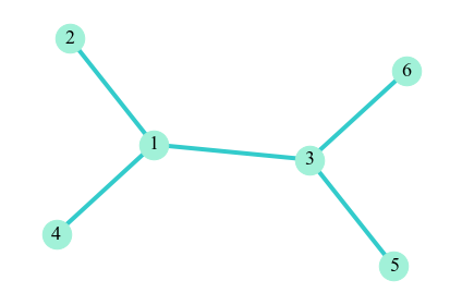
Graph Connectivity Problem
Since gPool omits nodes that are not in top $k$, their related edges will also be removed. As a result, the new graph formed by selected nodes will likely have isolated nodes. For example, take the graph below as the original graph
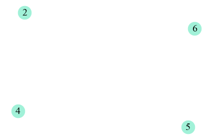
Suppose that gPool retains node $2, 4, 5$ and $6$, so node $1$, $3$ and their related edges wil be omitted. Then our new graph will be
In our new graph, the nodes are isolated. For GNN modules that aggregrate information from neighbor nodes, this could be a problem, since isolated nodes do not have neighbors to provide them information.
The authors of gPool solve this problem by using the power of the adjacency matrix. Specifically, in the Node Selection phase, instead of extracting rows and columns of the adjacency matrix $\mathbf{A}$ ($\mathbf{\hat{A}} = \mathbf{A}(\text{idx}, \text{idx})$), we can perform extraction from $\mathbf{A}^m$, i.e $ \mathbf{\hat{A}} = \mathbf{A}^m(\text{idx}, \text{idx})$. $\mathbf{A}^m$ builds connections between nodes whose distances are less than or equal to $m$, so using $\mathbf{A}^m$ can increase the connectivity of the new graph.
References
O. Vinyals, S. Bengio, and M. Kudlur. Order matters: Sequence to sequence for sets. In ICLR, 2015.
Jure Leskovec. Stanford CS224W: Machine Learning with Graphs, Lectur 8.
W.L. Hamilton. Graph representation learning. In Synthesis Lectures on Artifical Intelligence and Machine Learning, 14 (3) (2020), pp. 1-159.
H. Gao, S. Ji. Graph u-nets. In ICML, 2019.
R. Ying, J. You, C. Morris, X. Ren, W. Hamilton, and J. Leskovec. Hierarchical graph representation learning with differentiable pooling. In NeurIPS, 2018
D. Grattarola, D. Zambon, F.M. Bianchi, and C. Alippi. Understanding Pooling in Graph Neural Networks. arXiv preprint arXiv:2110.05292, 2021.